Table of Contents

Recap

The first part of this series introduced the notion of using a kernel to perform operations on image data. All of the examples used a 3x3 kernel that was aligned directly with the target pixel — this does not always have to be the case. This post will examine some additional kernel configurations, as well as the various parameters that can be tweaked when performing a convolution. These parameters are not necessarily part of the convolution operator itself, but are useful in many cases in which kernels and convolutions are used.

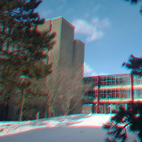
RGB Shifting, Component Extraction and Embossing - three of the many filters that use the parameters discussed in this post

Kernel Size

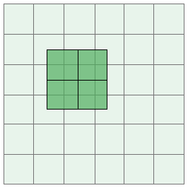
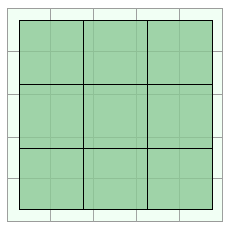
In theory, there are no restrictions on the size of a kernel. To be useful, however, a kernel should generally be small enough that the majority of the pixel accesses fall within the bounds of the target image. Consider the case of applying a 5x5 kernel to an 6x6 image:

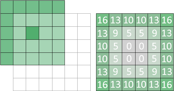
5x5 kernel applied to a 6x6 image; out of bounds access counts listed on the right

A large number of out of bounds accesses occur, which may or may not make the results of the kernel less meaningful. Another consideration, and perhaps the most important one, is performance. The output of a 9x9 Gaussian blur will look similar to an 11x11 Gaussian blur, but the 9x9 uses 40 fewer texture reads per pixel. In an OpenGL convolution shader it is likely that texture2D calls will be the bottleneck; the rest of the shader is just floating point arithmetic, which the GPU does very quickly. As such, a rule of thumb in real-time applications is to use the smallest possible kernel that produces the desired image. Kernel size can also be part of the user settings where applicable. A “low quality” bloom setting might use a 5x5 blur/bloom matrix, with the “high quality” option using a more expensive 9x9 kernel. For data centric applications that prioritize accuracy over speed, larger kernels may be more appropriate.

The easiest kernels to work with have two odd dimensions, such as 3x3, 5x5 or 7x11. This is because an odd dimension makes it possible to perfectly align the matrix with a target pixel as we’ve seen so far. A matrix with one or more even dimensions, such as 2x2 or 6x9 doesn’t have a central element:

2x2 kernel aligned with a target pixel

When applying a matrix with an even dimension there are two main conventions that can be used. The first is to simply mark one of the matrix entries as the “center” and align that element with the target pixel. The second option is to align the kernel as normal and apply a 0.5 pixel offset to each texture access. The offset an be implemented using the origin parameter described in the next section.

The half pixel option only works in systems with real-valued image access (such as textures in OpenGL or DirectX). The concept of a fractional pixel doesn’t exist when using raw image data stored in an array. Because of this the majority of image processing kernels have odd dimensions — when working on my convolution tool I didn’t run into a single even sized kernel.

Origin

The kernel origin or offset is another parameter that can be used to tweak the behavior of a convolution. After aligning the center of the kernel with the target pixel, the kernel is shifted by some amount in both the x and y directions. The kernel is convolved with the image at the new location, but the results are still stored at the original target location.

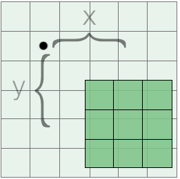
the x and y components of an origin used with a 3x3 kernel

If a constant origin is used for the whole image, the final output will appear to be shifted by the same factor. More interesting effects can be achieved by using an origin that varies per-pixel; for example, the origin could be chosen based on random noise or based on an image property such as pixel brightness or texture coordinates. An example of this is included in the convolution tool (note the distortion of certain features in the image):

Introducing an origin requires an update to the convolution equation listed in the previous post. The new expression is as follows, where o denotes the origin vector with components x and y:

The GLSL code can also be extended to include the origin parameter. To avoid duplicating the full shader multiple times, the snippet below lists a minimal example of the changes that are needed to add an origin parameter. A fully updated fragment shader that includes all of the new parameters is available at the end of the post.

...
uniform vec2 uTextureSize;
uniform vec2 uOrigin;
...
void main(void)
{
    ...
    vec2 stepSize = 1.0/(uTextureSize);
    vec2 coord = vTexCoord + uOrigin * stepSize;

    sum += texture2D(uSampler, vec2(coord.x - stepSize.x, coord.y - stepSize.y)) * uKernel[0];
    ...
}

The code above assumes that the uOrigin uniform is expressed as an pixel offset. Consequently, the value is scaled by stepSize to convert it to the same coordinate space as the texture coordinates.

Scale

The scale parameter is also used to change the way that a convolution fetches image data. The parameter increases the relative size of the kernel, making it cover a larger or smaller area of the image. The same number of texture accesses are performed, but their position is adjusted based on the scale parameter:

scale=1.0 on the left, scale=1.5 on the right

In a discrete system only integer scale values can be used, however in our shader implementation any floating point scale is possible. The scale is usually expressed as a two-component vector.

When using the scale parameter I found it was most useful to apply the scale first and then offset the pixel using the origin. The origin was therefore unaffected by the scale. It would be fairly easy to do the reverse and have the scale parameter also affect the origin. The updated convolution expression for the former case is as follows, where s is the scale vector:

This can be implemented in OpenGL quite easily by introducing a uScale uniform and multiplying it into stepSize:

...
uniform vec2 uTextureSize;
uniform vec2 uOrigin;
uniform vec2 uScale;
...
void main(void)
{
    ...
    vec2 stepSize = 1.0/(uTextureSize);
    vec2 coord = vTexCoord + uOrigin * stepSize;
    stepSize *= uScale;
    ...
}

To also apply the scale parameter to the origin, remove line #11 and include uScale directly in the stepSize computation:

vec2 stepSize = uScale/(uTextureSize);

Factor and Bias

Factor and bias are two additional floating point parameters that are used to scale the convolution output. Rather than changing the behavior of the operator itself, both parameters are applied outside of the convolution summation. The factor parameter is a scaling quantity that is multiplied by the result — bias is added on after the factor has been accounted for. The convolution equation can be extended to include a factor f and bias b as follows:

Technically the factor could be included in the kernel itself by multiplying each matrix entry by f. It is sometimes convenient to have it applied separately, however, and the extra multiplication has a negligible effect on shader performance. The bias parameter cannot be included in the kernel directly and must be implemented as an extra addition.

Factor and bias parameters are useful for remapping convolution output to a desired range. If a convolution returns values on the range [-1.0, 1.0] the results won’t display well if directly returned from a fragment shader. A factor of 0.5 and bias of 0.5 will map the output to the range [0.0, 1.0] which falls within the expected color range for OpenGL and DirectX shaders. An emboss filter is an example of this.

plain emboss filter on the left, emboss filter with a factor and bias of 0.5 on the right

The factor/bias parameters compress the output range of the convolution, but make the results visible — without including the parameters, all data on the range [-1.0, 0.0] would be clamped to a value of 0.0 by OpenGL. For applications that can write to a full-range floating point texture, this use of factor and bias may not apply.

Adding the parameters to our convolution shader can be done as follows:

...
uniform vec2 uScale;
uniform float uFactor;
uniform float uBias;
...
void main(void)
{
    ...
    sum = sum * uFactor + uBias;
    sum.a = 1.0;
    gl_FragColor = sum;
}

Normalization

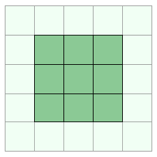
Normalization is an optional step that can be applied to a kernel in order to bound the output, usually to achieve a maximum value of one. Consider the following kernel:

If the kernel is convolved with an image the output can fall anywhere on the range [0.0, 9.0]. If all nine of the pixels sampled had a value of 1.0, for example, applying the kernel would cause the target pixel to become over saturated. This is generally not desirable — the above kernel is an example of a smoothing filter that’s used to blur images, not for increasing brightness.

To remedy this issue the kernel elements can be normalized by dividing each matrix element by the absolute value sum of all elements:

In the above expression, K is an mxn kernel. The resulting matrix is the same size as the original, but the output range will be constrained to [0.0, 1.0]. After normalization, the smoothing kernel listed above would look like:

Although useful in some cases, it is not always necessary to normalize a kernel. Some kernels, like the edge detector from the previous post, have elements that naturally sum to 0 instead of 1.

Normalization can be implemented using the factor parameter discussed in the previous section. Alternatively, a kernel could be normalized before passing the data to a convolution shader. In both of these cases no changes are needed to the shader itself.

Component Splitting

Many images are composed of multiple color components, such as RGB or CMYK. Thus far the kernels we’ve looked at are applied uniformly across the image data — the same kernel and parameters are used for all of the color channels. It is possible to use different kernel and parameter values for each of the components in the image.

Splitting up kernel data, factor and bias on a per-component basis is relatively straightforward. The uKernel, uFactor and uBias uniforms need to be changed to the vec3 or vec4 type depending on the number of color channels. OpenGL and DirectX support component-wise multiplication of vector data, so the following will work as expected:

...
uniform vec3 uKernel[9];
uniform vec3 uFactor;
uniform vec3 uBias;
...
void main(void)
{
    sum += texture2D(uSampler, vec2(coord.x - stepSize.x, coord.y - stepSize.y)) * uKernel[0];
    ...
    sum = sum * uFactor + uBias;
    ...
}

The only change needed is the type on the uniform inputs. Things get more complicated when implementing a per-component origin or scale. This requires separate texture2D calls per component, since each component will be sampling the source image at different locations. I haven’t tried this myself, but something like the following should work for a custom origin and scale:

...
uniform vec3 uKernel[9];
uniform vec2 uOrigin[3];
uniform vec2 uScale[3];
...
void main(void)
{
    vec2 stepSize = 1.0/(uTextureSize);

    vec2 coordR = vTexCoord + uOrigin[0] * stepSize;
    vec2 coordG = vTexCoord + uOrigin[1] * stepSize;
    vec2 coordB = vTexCoord + uOrigin[2] * stepSize;

    vec2 stepR = stepSize * uScale[0];
    vec2 stepG = stepSize * uScale[1];
    vec2 stepB = stepSize * uScale[2];

    sum.r += texture2D(uSampler, vec2(coord.x - stepR.x, coord.y - stepR.y)) * uKernel[0].r;
    sum.g += texture2D(uSampler, vec2(coord.x - stepR.x, coord.y - stepR.y)) * uKernel[0].g;
    sum.b += texture2D(uSampler, vec2(coord.x - stepR.x, coord.y - stepR.y)) * uKernel[0].b;

    ...
}

Keep in mind that this approach is more expensive as the number of texture fetches is now scaled by the number of color channels in the image.

Shader code

The final code for the parameters discussion in this section, excluding RGB splitting, is listed below. The basic RGB splitting can be added by changing the float parameters uKernel, uFactor and uBias to vec3 parameters. RGB splitting for uOrigin and uScale is left as an exercise for the reader — if you want to discuss it in more detail, feel free to contact me. I am curious to see what sort of optimizations can be made and what applications require that particular feature.

uniform sampler2D uSampler;

uniform float uKernel[9];
uniform vec2 uOrigin;
uniform vec2 uScale;
uniform float uFactor;
uniform float uBias;

uniform vec2 uTextureSize;

varying vec2 vTexCoord;

void main(void)
{
    vec4 sum = vec4(0.0);

    vec2 stepSize = 1.0/(uTextureSize);
    vec2 coord = vTexCoord + uOrigin * stepSize;
    stepSize *= uScale;

    sum += texture2D(uSampler, vec2(coord.x - stepSize.x, coord.y - stepSize.y)) * uKernel[0];
    sum += texture2D(uSampler, vec2(coord.x, coord.y - stepSize.y)) * uKernel[1];
    sum += texture2D(uSampler, vec2(coord.x + stepSize.x, coord.y - stepSize.y)) * uKernel[2];

    sum += texture2D(uSampler, vec2(coord.x - stepSize.x, coord.y)) * uKernel[3];
    sum += texture2D(uSampler, vec2(coord.x, coord.y)) * uKernel[4];
    sum += texture2D(uSampler, vec2(coord.x + stepSize.x, coord.y)) * uKernel[5];

    sum += texture2D(uSampler, vec2(coord.x - stepSize.x, coord.y + stepSize.y)) * uKernel[6];
    sum += texture2D(uSampler, vec2(coord.x, coord.y + stepSize.y)) * uKernel[7];
    sum += texture2D(uSampler, vec2(coord.x + stepSize.x, coord.y + stepSize.y)) * uKernel[8];

    sum = sum * uFactor + uBias;
    sum.a = 1.0;
    gl_FragColor = sum;
}

Wrap Up

In addition to the parameters discussed in this post, plenty of other interesting things can be done to alter the way kernels are applied. A kernel could be rotated or skewed, for example. The case can be made for performing pretty much any affine transformation to the base kernel with respect to the target location in the image.

In Part 3 we’ll take a look at some examples of commonly used image filters, their applications and the way the kernels are derived.