Train Control Project

At the beginning of the month my partner and I completed the kernel portion of our CS 452 coursework. We’ll be spending the remainder of the term implementing a train control system that runs on our OS. The goal is to develop a unique project that demonstrates all of the work we’ve done in the course.

The control system is broken into three major parts, each of which is presented to the course staff. The first milestone is position and velocity tracking, as well as stopping distance prediction. Only a single train needs to be on the track for the first component; scheduling and collision avoidance are part of the second milestone. The specifics of the final component are left up to the student teams. The only requirement is that the demo makes use of path planning and tracking functionality. In the past teams have created games like Snake or Pac-Man with the trains, or taken on ambitious scheduling tasks like running five trains concurrently.

We gave our first demo last week, after several days of calibration and testing. In the demo the train operated at max speed and traversed a variety of different routes on the track. To showcase position and velocity tracking, the system reported the expected arrival time of the train at each of the sensors along its path. We also included a command to stop the train at a known location, such as a sensor node. Since the train has inertia and can coast for over a meter before coming to a complete stop, the control system had to estimate deceleration time to determine when to issue the stop command.

A train stopping on top of a sensor

Track Data and Measurements

Before writing code to control the trains, accurate measurements of the track layouts were needed. Each of the two layouts in the CS 452 lab consists of hundreds of individual segments and twenty-two switch modules. The segments come in a variety of different shapes and sizes, including curved pieces of different radii. The main portion of the track forms a figure-8 shape with a larger loop around the outside. The loops funnel into a collection of straight segments that can be used to park trains:

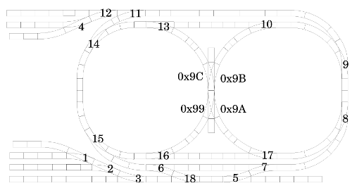
One of the track configurations, including switch IDs

Segment lengths in millimeters are published by the train set manufacturer, however sorting through all the information is a time consuming task. A group of students that took CS 452 several years ago created a graph data structure based on the track spec. Their code is available on the course website and is the recommended way to query track distances.

The data structure is a bidirectional graph of all of the track segments, including sensors and switches. The graph can be used to query the distance between pairs of sensors, or to determine the ID of the next sensor or switch on a train’s route.

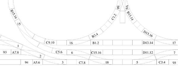
A close-up of part of the track - sensor nodes begin with a letter.

Code for traversing the graph has to be written from scratch — searching and path planning algorithms aren’t included in the data structure. This aspect of the control system was my partner’s responsibility, while I focused on collecting train data, modeling and calibration techniques.

One of the challenges with interacting with the track is that we’re expected to handle sensor and switch failure. My partner designed a robust system that allows us to miss every other sensor without losing track of where the train should be heading. We don’t need to handle double sensor failures for the course, and so far none of the tracks have pairs of broken sensors.

The controller is also able to handle broken switches by assuming that the train takes both of the potential switch paths. A future sensor read confirms with of the paths was actually taken and the controller discards the data for the path that was not.

Modeling Challenges

The biggest challenge when simulating the physics of a train is that the train hardware doesn’t offer a mechanism to query train speed or displacement. Internally the train uses a feedback controller to achieve the desired velocity, however the controller isn’t always able to maintain constant, predictable state. The details of the controller aren’t public available either, so we had to collect data and develop a model ourselves.

The speed sent to the train is an arbitrary, unitless quantity on the range [0,14]. A speed of zero indicates that the train should stop, while other speeds increase the trains velocity in non linear increments. The course material, and my blog posts, refer to this unitless quantity as “train speed”. The actual velocity of the train in the physical world is referred to as “velocity”.

Various changes in the train and track result in accelerations that affect train velocity. The most obvious is changing speeds, such as going from speed 5 to 14 or from 12 to 0. Going around a curved segment also causes some loss in speed, most likely due to centripetal force and the curved shape track resulting in higher friction on the wheels.

Velocity is also lost when the train travels over a “dead zone”, which is an area of the track were the voltage pickups are damaged. The train is momentarily unpowered on these regions, and therefore slows down as it coasts back into a region with a proper power supply. Both of the tracks in the lab have several dead zones, and one of the tracks has a damaged segment that can only be traversed in one direction. These problems are periodically fixed by the course staff, however it is expected that student projects are able to handle tracks with a reasonable number of dead zones.

Another source of error comes from problems in the timing systems and hardware. Like all electronics, there is a limit to how fast commands can be sent to the train hardware. The connection uses a baud rate of 2400. Each character sent has 1 start bit and 2 stop bits for a total of 11 bits for each byte command. There is an upper limit of 218 commands per second; since some of the commands require multiple bytes and send response data back, in the practice the value is much smaller.

Data Collection

Developing a physical model for the trains required a large amount of data. To reduce systemic error during data collection, I wrote a calibration tool that runs directly on the hardware. The tool polls a pair of sensors on the track and reports the time taken between the sensors firing. These measurements were used as the basis for all of our data collection.

Steady State Velocity

Steady state velocity was by far the easiest quantity to measure. The physical distance between any two sensors can be found using the track data graph; along with the timing measurements this is sufficient information to compute velocity:

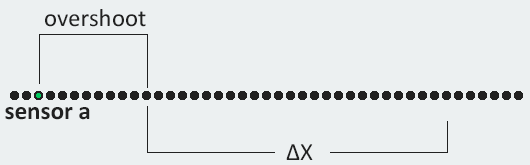
The overshoot problem discussed previously is a non-factor in the steady velocity calculation, since it offsets both the start and end sample times. The timing error from overshoot therefore cancels out.

The above equation implies that the overshoot error is the same on both ends, which is not always the case. In pratice, however, it was a safe assumption to make since our calibration averaging multiple velocity samples.

Experimental setup for measuring steady state velocity

Data collection for velocity consisted of taking around 20 timing samples for each of the non-zero train speeds. The process took around an hour to complete, however once the collection program was launched it was more or less automatic. At low speeds the train occasionally got stuck on dead spots, and required a nudge to continue operating.

Stopping Acceleration

Measuring the stopping acceleration of the trains was more challenging, since the stopping distance of the train wasn’t the same as the distance between sensor pairs. This meant that there was no reliable way to report the time taken to decelerate to a physical speed of 0. However, since a model for velocity had already been determined, we were able to use kinetic energy to estimate the amount of force applied to stop the train. Fortunately mass cancels out on both sides, thus avoiding the need to weigh each train:

During data collection the train was set to a pre-determined speed; the value of v was computed based on that speed setting. A stop command was then sent to the train when it passed a sensor, and the stopping distance x was measured using a piece of string and a ruler. The energy equation was then used to solve for stopping acceleration.

The problem with this technique was that overshoot and command processing delay affected the measurements of x. To compensate for the error, we needed to know how far the train traveled past the sensor before it received a stop command.

Experimental setup for measuring stopping distance

The overshoot measured by running the train over a sensor and turning on the front headlights as soon as the sensor was triggered. Video was taken of the procedure, and stepped through frame-by-frame to estimate the delay between crossing a sensor and turning on the lights. In the initial experiment we measured overshoot distance, which was then later converted to overshoot time. The measurements indicated that there was a delay of between 100 and 200 ms, depending on various random factors.

Transfer Acceleration

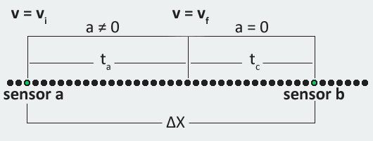
Experimental setup for measuring transfer acceleration

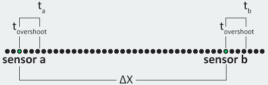
Measuring the acceleration when moving between two non-zero speeds required clever use of kinematic equations. Like the steady state velocity, we started by measuring the time delta between a pair of sensors. As seen in the diagram above, the total time between the two sensors is t. At some point between them, labeled as t_a, the train has reached the target velocity. At this point the train has reached the target velocity and stops accelerating, for a time of t_c. The time delta is the sum of the two:

The kinematics for the train can be expressed as follows:

The second equation can be rearranged to solve for a:

Subbing in for a in the first equation, and writing t_c in terms of t_a:

The only unknown is t_a, since the steady state speeds v_i and v_f were founded earlier. The position and time deltas are measured directly by the calibration system. Once the acceleration time is found, acceleration velocity can be computed using the rearranged form of equation 2 listed earlier:

The same experimental setup was used to find starting acceleration, since it’s a special case of the above derivation with v_i set to zero. It is worth noting that overshoot handling is also necessary when measuring transfer acceleration since the overshoot distance is different on both ends. On the initial edge the overshoot distance is v_i*t_overshoot, while on the opposite end the distance is v_f*t_overshoot.

Physical Model

Static Model

We were allowed to select our track, switch configuration and train for Demo 1, so I saved some time by only generating a model for one of the trains. The train tracks its current velocity and acceleration based on the the speed commands; every time a speed command is sent to the track hardware, a similar command is sent to the train physics code. The physics also records the total distance traveled. A time step of 10ms is used to advance the simulation, which involves updating the velocity and position.

The static model is able to respond to a variety of queries that related to the functional we need for the train controller. For example, the model can return the stopping distance given the current train state, or compute the time need to travel a certain distance.

Dynamic Model

On its own, the static model ended up being a poor predictor of the train position and velocity. This wasn’t really surprising, given what we knew about the train set. Run time alterations to the model were needed to account for variations in the track, train and hardware timing.

The first dynamic refinement method I implemented was to recompute the current velocity every time the train passed over a sensor. The time taken between sensors was recorded and the sensor distance was found using the graph data structure. To avoid making large, potentially erroneous changes to the velocity model, the new velocity was added onto the model using a weighted average:

This technique helped the train controller to correct for low frequency changes in velocity, such as the train running slower due to temperature or friction in the mechanics.

A second, finer-grain technique was needed to handle issues like damaged switches, dead zones or sticky track segments. At every sensor the train controller makes a prediction for the arrival time at the next sensor on the route. Upon reaching that sensor, the prediction error is computed and used to determine a velocity loss coefficient. Rather than storing the coefficient in the train controller, it gets stored directly onto the graph edge between the two sensors. Future physics computations involving that edge make use of the error term to correct for deviations in velocity.

Model Performance

During our demo the train operated at a velocity of roughly 52 cm/s. After building a stable set of dynamic calibration values, sensor predictions were almost always within 30ms of the measured time. This translates into a maximum error of around 1.56 cm in the position tracking.

For the stopping distance demo we allowed our professor to specify a location on the track for the train to stop at. We were able to track the train well enough to stop within a few centimeters of the chosen location on all three of the tests we ran during the presentation.